Excel Charting Elements
|
|
|
|
|
|
|
|
|
|
|
|
|
|
Additional Resources
Excel Charting Elements | Microsoft Excel XP |
 |
Dealing With Chart Elements
Working with Excel charting elements in a chart is similar to everything else you do in Excel: First you make a selection (in this case, select a chart part), and then you issue a command to do something with the selection.You can activate a chart element in any of three ways:
| ► | Click the chart element. |
| ► | Press the up-arrow or down-arrow key to cycle
through all the elements in the chart. When a data series is selected, you can press the right-arrow or left-arrow key to select individual points in the series. |
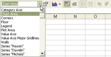
| ► | Use the Chart Objects control in the Chart
toolbar. This is a drop-down list that contains all of the elements in the chart. |
 |
No matter which method you use, the name of the selected item appears in the Name box (at the left of the formula bar).
Many of the Excel charting elements' names include a number that further describes the element.
For example, the third point of the first data series is named Series 1 Point 3.
You cannot change the names of Excel charting elements, and you cannot select more than one Excel charting elements at a time.
 |
When you move the mouse pointer over any of the Excel charting elements, a chart tip displays the name of the element. If the element is a data point, the chart tip displays the value. To control what appears in these chart tips, use the Tools ► Options command and click the Chart tab. Make your selection in the Chart tips section of the dialog box. |
Modify A Chart Element
Most Excel charting elements can be modified in several ways. For example, you can change colors, line widths, fonts, and so on. Modifications are made in the Format dialog box (which varies for each type of chart element).To modify an element in a chart, follow these steps:
| 1. | Select the chart element. |
| 2. | Access the Format dialog box using any of the following techniques: |
| ► Double-click the item. | |
| ► Choose the Format ► [item name] command. | |
| ► Press CTRL + 1 | |
| ► Right-click the item and choose Format [item name] from the shortcut menu. | |
| 3. | Click the tab that corresponds with what you want to do. |
| 4. | Make the changes. |
| 5. | Click OK. |
Excel XP Topics
- Tips- Excel Screen Layout
- Navigational Techniques
- Working with Workbooks
- Templates
- Working with Worksheets
- Moving Around
- Move Worksheets
- Copy Worksheets
- Insert & Delete Cells
- Insert & Delete Rows
- Insert & Delete Columns
- Resize Row
- Resize Column
- Editing Data
- Content Color
- Cell Color
- Number Formats
- Fonts
- Alignment
- Text Direction
- Indent Contents
- Merge Cells
- Copy
- Move
- Undo & Redo
- Using Zoom
- Freeze & Unfreeze Titles
- Split Worksheet
- Spreadsheet Data
- AutoFill
- AutoComplete
- Comment
- Find
- Replace
- Spellcheck
- Formulas
- Functions
- Password
- Sorting
- AutoFilter
- Advanced Filter
- Macros
- Charts
- Charting
- Charting Elements
- Gantt Chart
- PivotTable
- PivotTable Calculations
- PivotTable Layout
- PivotTable Format
- PDF to Excel
- PDF-to-Excel Converter
- Excel to PDF Converter